Hands on Machine Learning

ai #ml #books

Chapter 1

When to Use Machine Learning

Machine learning (ML) can be a powerful tool, but it’s not always the best solution. Understanding when to use ML and when not to depends on the nature of the problem, the data available, and the desired outcomes. Here’s a breakdown of when you should consider using ML and when you might want to opt for traditional programming or other methods.

When to Use Machine Learning

1. When There is a Need to Make Data-Driven Predictions:

   • Use Case: Predicting stock prices, estimating house prices, or customer churn prediction.
   • Rationale: ML models excel at making predictions based on patterns in historical data, enabling accurate forecasting in scenarios with complex relationships between variables.

2. When the Problem Involves Complex Patterns or Non-Linear Relationships:

   • Use Case: Image recognition, natural language processing (NLP), and speech recognition.
   • Rationale: Problems involving complex, non-linear relationships or unstructured data (e.g., images, audio, text) are challenging to solve with rule-based approaches. ML models can detect subtle patterns in such data that would be difficult or impossible to encode manually.

3. When Manual Feature Engineering or Rules Are Impractical:

   • Use Case: Identifying spam emails, classifying products in an e-commerce catalog.
   • Rationale: For problems that require hundreds or thousands of rules or for scenarios where these rules constantly change, using ML can automate feature extraction and pattern recognition.

4. When You Need to Personalize User Experiences:

   • Use Case: Personalized recommendations (e.g., Netflix, Amazon), targeted advertisements.
   • Rationale: ML models can learn user preferences and behavior over time, providing personalized recommendations and improving user engagement.

5. When the System Needs to Adapt Over Time:

   • Use Case: Fraud detection systems, dynamic pricing models.
   • Rationale: Some systems must adapt to changes in user behavior, data patterns, or the environment. ML models can be updated regularly with new data, making them ideal for dynamic and evolving systems.

6. When Handling Large Amounts of Unstructured Data:

   • Use Case: Sentiment analysis, summarization of large documents, automatic tagging of images.
   • Rationale: Unstructured data (e.g., text, images, videos) often cannot be easily handled with traditional algorithms. ML models, particularly deep learning, can process and extract insights from these data types effectively.

When NOT to Use Machine Learning

1. When the Problem Can Be Solved with Simple Rules:

   • Example: Validating email addresses, basic arithmetic operations.
   • Rationale: If the problem can be defined using straightforward if-else rules or regular expressions, using ML adds unnecessary complexity and resource consumption.

2. When You Don’t Have Enough or Good Quality Data:

   • Example: Predicting sales with very few data points or with incomplete data.
   • Rationale: ML models rely heavily on data to learn patterns. Without sufficient data, the model is likely to overfit or produce unreliable results. It’s better to first focus on collecting more data or improving data quality before applying ML.

3. When Interpretability and Transparency are Crucial:

   • Example: Legal decision-making, medical diagnosis.
   • Rationale: Some ML models, like deep learning networks, act as “black boxes” and offer little interpretability. In scenarios where understanding the decision-making process is critical, using traditional, interpretable methods (e.g., rule-based systems or linear models) might be more appropriate.

4. When There Are No Clear Performance Metrics or Objectives:

   • Example: Exploring a new problem without knowing what to optimize for.
   • Rationale: ML models require well-defined metrics to evaluate their performance. If the problem’s success criteria are unclear or not measurable, it’s better to refine the problem statement and objectives first.

5. When the System Needs to Operate with Low Latency and Limited Resources:

   • Example: Real-time systems with strict performance constraints.
   • Rationale: ML models can be computationally intensive and may not meet the performance requirements of real-time systems, especially if resources like CPU or memory are limited. In such cases, lightweight algorithms or rule-based approaches may be more suitable.

6. When the Cost of Error is Extremely High:

   • Example: Autonomous driving, high-stakes financial trading.
   • Rationale: ML models are probabilistic and can produce erroneous outputs. In situations where errors can result in significant damage, loss, or risk to human life, using deterministic methods or combining ML with strong safety mechanisms is recommended.

7. When Legal, Ethical, or Privacy Concerns Are a Priority:

   • Example: Using personal data for predictive modeling without clear user consent.
   • Rationale: ML often requires large amounts of data, and using this data can pose ethical and legal issues, particularly if it involves sensitive information. In such cases, it’s better to avoid ML or ensure strict adherence to legal and ethical guidelines (e.g., GDPR compliance).

Deciding Factors

Here are a few questions to ask when deciding whether to use machine learning:

1. Can the problem be defined clearly with rules? If so, use traditional programming.
2. Is there sufficient quality data available? If not, focus on data collection first.
3. Does the problem require adaptability over time? If yes, ML can be beneficial.
4. Is interpretability crucial? If yes, consider rule-based methods or simpler models like linear regression.
5. Are there strict performance constraints? If yes, evaluate whether ML models can meet them.

In summary, machine learning should be used when traditional programming falls short due to the complexity or dynamic nature of the problem, and when there is sufficient high-quality data to support the model’s learning process.

ML Model Development Phases

The development of a machine learning model typically involves several structured phases to ensure the model’s efficacy and robustness. These phases are as follows:

1. Problem Definition and Scope

• Define the Objective: Clearly articulate what problem the model aims to solve and the expected outcome.
• Understand Business Constraints and Requirements: Identify any business or technical constraints, such as computational resources, latency, or regulatory requirements.
• Determine Evaluation Metrics: Choose appropriate metrics (e.g., accuracy, precision, recall, F1 score) that will be used to measure the model’s performance.

2. Data Collection and Understanding

• Identify Data Sources: Determine where data will be sourced from (internal databases, external APIs, etc.).
• Data Acquisition: Collect the data needed for model training and testing.
• Exploratory Data Analysis (EDA): Gain insights into the data by analyzing patterns, distributions, correlations, and anomalies.
• Understand Data Quality: Check for missing values, inconsistencies, and data imbalances.

3. Data Preprocessing

• Data Cleaning: Handle missing values, outliers, and errors in the data.
• Feature Engineering: Create new features or transform existing ones to better capture the underlying patterns. This can include scaling, normalization, encoding categorical variables, and generating polynomial features.
• Feature Selection: Select the most relevant features using techniques such as variance thresholding, mutual information, or recursive feature elimination.
• Data Splitting: Split the data into training, validation, and test sets to evaluate model performance and generalization.

4. Model Selection

• Choose Model Type: Decide on the type of model based on the problem (e.g., regression, classification, clustering, or time series forecasting).
• Select Algorithms: Evaluate different algorithms (e.g., linear regression, decision trees, SVM, neural networks) that are well-suited for the chosen model type.
• Baseline Model Creation: Create a simple model to establish a baseline performance for comparison.

5. Model Training

• Train the Model: Use the training data to train different models and adjust hyperparameters.
• Hyperparameter Tuning: Optimize model parameters using techniques such as grid search, random search, or Bayesian optimization.
• Cross-Validation: Use k-fold cross-validation to reduce the risk of overfitting and validate model performance.

6. Model Evaluation

• Evaluate on Validation Set: Assess the model using the validation set and chosen evaluation metrics.
• Error Analysis: Analyze the errors made by the model to identify patterns and areas of improvement.
• Comparison Against Baseline: Compare the model’s performance against the baseline to ensure that it offers a significant improvement.

7. Model Optimization

• Address Overfitting or Underfitting: Adjust the model’s complexity, add regularization, or obtain more data to address performance issues.
• Model Simplification: Consider reducing model complexity to enhance interpretability and reduce computational costs.
• Feature Importance Analysis: Analyze feature importance to understand which features are contributing most to the model’s predictions.

8. Model Deployment

• Deployment Strategy: Choose an appropriate strategy for deploying the model (e.g., batch, real-time, or streaming).
• Containerization and Integration: Package the model using tools like Docker and integrate it with the application infrastructure.
• Monitoring and Logging: Set up monitoring and logging to track model performance, identify drift, and trigger re-training if necessary.

9. Model Maintenance and Continuous Improvement

• Performance Monitoring: Continuously monitor model performance in production and detect issues such as data drift or model degradation.
• Re-Training and Versioning: Update the model with new data or improved techniques and maintain version control.
• Feedback Loop Implementation: Collect feedback from users or stakeholders to enhance the model’s performance and adapt it to evolving requirements.

By following these phases systematically, the development and deployment of machine learning models become more structured, resulting in models that are not only performant but also maintainable and adaptable to changing environments and requirements.

Importance of Data

The referenced excerpt discusses a significant finding in the field of machine learning, where different machine learning algorithms (even relatively simple ones) tend to perform almost equally well on complex problems, provided that they are supplied with sufficient data. This insight was initially observed by Eric Brill and later popularized by Peter Norvig and his co-authors in their 2009 paper titled “The Unreasonable Effectiveness of Data.”

The main message of this paper is that, in many cases, having a large volume of high-quality data can be more crucial to the success of a machine learning model than the choice or sophistication of the algorithm itself. This finding suggests that for complex problems like natural language processing, the focus should perhaps shift from algorithmic innovation to gathering and curating large datasets.

However, the paper also notes that in real-world scenarios, large datasets may not always be readily available due to cost or accessibility constraints, and small- to medium-sized datasets are still prevalent. Thus, while data is undeniably crucial, the choice of algorithm remains relevant and should not be disregarded when working with limited data.

In summary, the paper advocates for a balanced approach, recognizing the importance of both data and algorithms, but emphasizing that in many complex problems, more data can often compensate for less sophisticated algorithms.

What is the difference between a model parameter and a learning algorithm’s hyperparameter?

In the context of machine learning:

Model Parameters:

• Definition: Model parameters are the internal variables of the model that are learned from the training data during the training process.
• Purpose: These parameters define the model’s structure and are adjusted to minimize the error or loss function.
• Examples: In a linear regression model, the coefficients (weights) and intercept are model parameters. In a neural network, the weights and biases of each neuron are considered model parameters.
• Characteristic: Model parameters are determined automatically by the learning algorithm and directly influence the model’s predictions.

Hyperparameters:

• Definition: Hyperparameters are external configurations set before the learning process begins. They control the behavior of the learning algorithm and the overall model architecture.
• Purpose: They are used to guide the training process, influencing how the model learns from data.
• Examples: Learning rate, number of hidden layers in a neural network, regularization strength, batch size, and number of iterations are typical hyperparameters.
• Characteristic: Hyperparameters are not learned from the data. Instead, they are set manually or through methods like grid search or random search. Hyperparameters influence the performance and complexity of the model, but they do not change during the model training.

Summary:

• Model parameters are learned by the model during training and define the model’s predictive capabilities.
• Hyperparameters are set before training and determine how the learning process is carried out, affecting model optimization and architecture.

Understanding and correctly tuning hyperparameters is crucial for optimizing model performance and ensuring that the learning algorithm converges effectively on the desired solution.

If your model performs great on the training data but generalizes poorly to new instances, what is happening? Can you name three possible solutions?

If your model performs well on the training data but generalizes poorly to new instances, it is likely overfitting. Overfitting occurs when the model learns not only the underlying patterns in the training data but also the noise and outliers, causing it to perform poorly on unseen data.

Three Possible Solutions to Overfitting:

1. Reduce Model Complexity:

   • Simplify the model by using fewer features or reducing the number of layers or neurons in a neural network.
   • Use a less complex algorithm (e.g., replace a high-degree polynomial model with a lower-degree one).

2. Regularization:

   • Apply regularization techniques like L1 (Lasso) or L2 (Ridge) regularization to add a penalty to larger coefficients, encouraging the model to generalize better.
   • Use dropout in neural networks to randomly deactivate a subset of neurons during training, preventing over-reliance on specific paths.

3. Increase the Training Data:

   • Gather more training data or use data augmentation techniques to create variations of existing data (e.g., flipping, rotating, or scaling images).
   • This helps the model learn broader patterns and reduces the risk of overfitting to a small set of examples.

Each of these techniques helps improve generalization and ensures that the model performs well on both training and unseen data.

What is repeated cross-validation and why would you prefer it to using a single validation set?

Repeated Cross-Validation:

Repeated cross-validation is a method that involves applying the cross-validation procedure multiple times. It splits the dataset into different training and validation sets in each repetition and averages the results across these repetitions. A common approach is to perform k-fold cross-validation multiple times (e.g., 10 times with 10 different splits), where the data is divided into k folds, and the model is trained and validated k times, each time using a different fold as the validation set.

Why Prefer Repeated Cross-Validation Over a Single Validation Set:

1. More Reliable Performance Estimation:

   • Repeated cross-validation provides a more robust and reliable estimate of model performance because it averages the results over multiple different splits of the data, reducing the variance caused by random variations in a single split.

2. Reduced Risk of Overfitting to the Validation Set:

   • Using a single validation set can lead to overfitting on that particular set, especially if the dataset is small. Repeated cross-validation mitigates this risk by validating the model on multiple subsets of the data.

3. Better Utilization of Data:

   • Repeated cross-validation makes better use of the available data because every observation is used for both training and validation multiple times. This is particularly beneficial when the dataset is small, as it ensures that no single point is left out of the model building for too long.

Summary:

Repeated cross-validation provides a more stable and reliable estimate of a model’s generalization performance by reducing variance and better utilizing the data. It is preferable to using a single validation set, especially in scenarios where data is limited or when the model’s performance needs to be evaluated more rigorously.

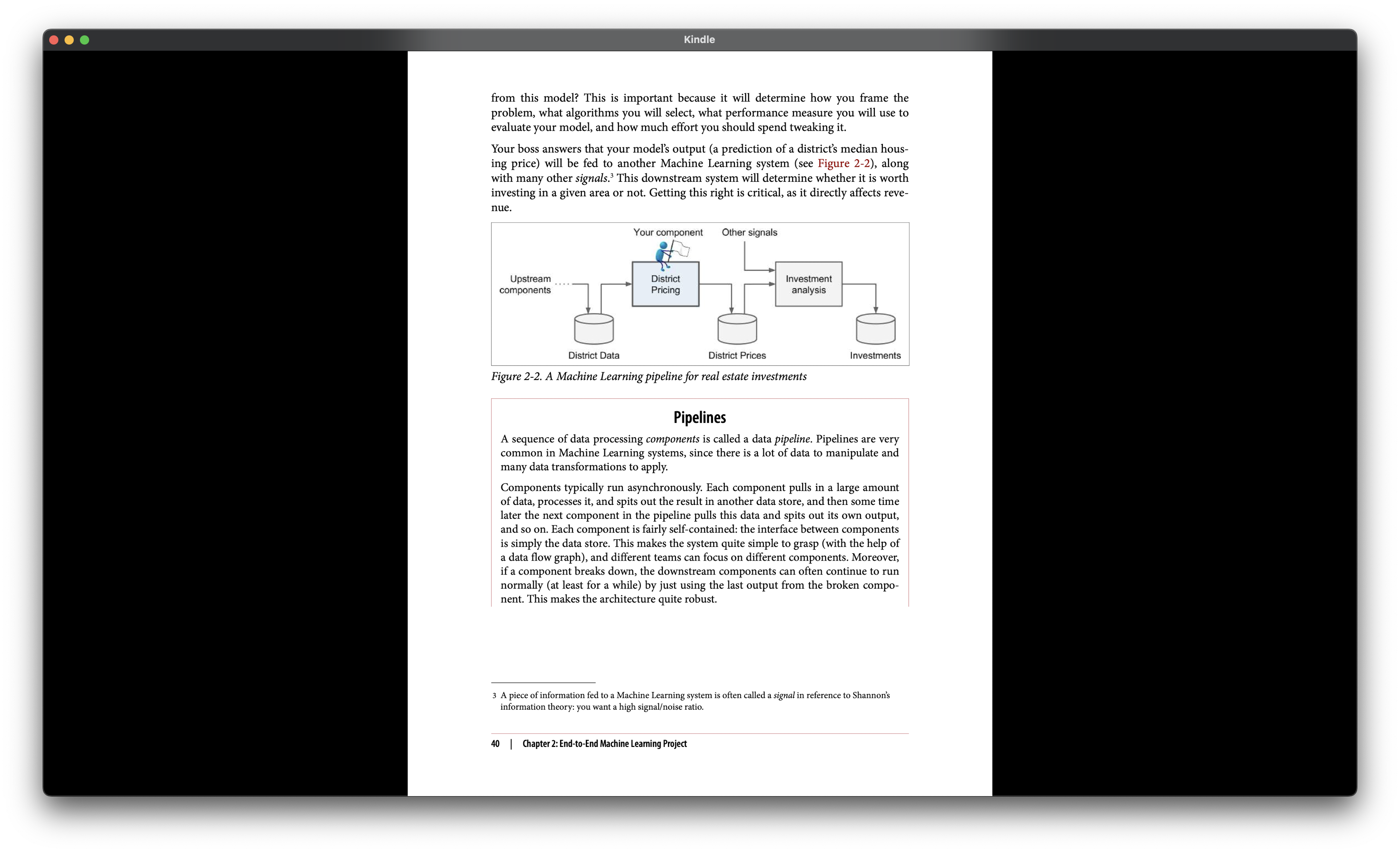
CH2 End-to-End Machine Learning Project

The excerpt outlines a structured 8-step process for developing and deploying a machine learning project. Here’s a brief explanation of each step:

1. Look at the Big Picture

• Define the problem clearly, understand the business objectives, and determine how machine learning can help. Set the project’s goals, success criteria, and constraints.

2. Get the Data

• Identify and gather the data required for the project. This can involve accessing databases, collecting data from APIs, or other sources. Ensure the data is relevant and sufficient for the problem at hand.

3. Discover and Visualize the Data to Gain Insights

• Perform exploratory data analysis (EDA) to understand the data’s structure and patterns. Use statistical analysis and visualization techniques to identify correlations, anomalies, and key features.

4. Prepare the Data for Machine Learning Algorithms

• Clean and preprocess the data by handling missing values, scaling features, encoding categorical variables, and performing feature engineering. Split the data into training and test sets.

5. Select a Model and Train It

• Choose a suitable machine learning model or algorithm based on the problem type (e.g., classification, regression). Train the model using the training data.

6. Fine-Tune Your Model

• Optimize the model by tuning hyperparameters and performing cross-validation. Try different models or ensemble methods to find the best-performing solution.

7. Present Your Solution

• Summarize your findings and the performance of the model. Present results in an easily understandable format for stakeholders, along with any insights derived from the analysis.

8. Launch, Monitor, and Maintain Your System

• Deploy the model into a production environment. Monitor its performance, retrain or update the model as necessary, and handle any issues that arise during operation. Ensure the system adapts to changing data or requirements over time.

This comprehensive process provides a systematic approach to building, evaluating, and deploying machine learning solutions effectively, covering the entire machine learning workflow from data acquisition to deployment and maintenance.

Training with Big data if not fit to memory

The excerpt discusses strategies for handling large datasets when training machine learning models. When the data is too large to fit in memory or be processed in a single batch, two common techniques can be used:

1. Distributed Batch Learning (e.g., Using MapReduce):

• In batch learning, the entire dataset is used to train the model at once, which can be computationally intensive when dealing with large datasets. One approach to handling this is to distribute the computation across multiple servers using techniques like MapReduce. MapReduce allows the dataset to be split into smaller chunks, which are processed in parallel on different servers (the “Map” step). The results are then combined and aggregated (the “Reduce” step). This makes it possible to train models on massive datasets more efficiently by leveraging distributed computing resources.

2. Online Learning:

• Online learning involves training the model incrementally by feeding it data one instance (or mini-batch) at a time. This technique is particularly useful for large datasets because it doesn’t require loading the entire dataset into memory. Instead, the model updates itself iteratively as new data arrives. Online learning is also effective for models that need to adapt to rapidly changing data or scenarios where the data is generated continuously (e.g., real-time data streams).

Summary:

• Distributed Batch Learning (using techniques like MapReduce) is suited for processing large datasets by splitting the work across multiple servers.
• Online Learning is beneficial when the dataset is too large to fit in memory or when the model needs to adapt incrementally to new data points.

These strategies allow machine learning models to be trained effectively on huge datasets that would otherwise be difficult to handle with standard batch learning techniques.

Performance measure for Regression

Performance measures for regression algorithms help evaluate how well the model predicts continuous outcomes. Here are some common performance metrics used for regression tasks:

1. Mean Absolute Error (MAE)

• Formula: $$\text{MAE}=\frac{1}{n}\sum _{i=1}^n|y_i-{\hat{y}}_i|$$
• Description: Measures the average magnitude of errors between the predicted and actual values without considering their direction. It is less sensitive to outliers compared to other metrics like MSE.
• Use Case: Useful when all errors have the same importance, and you want a simple measure of prediction accuracy.

2. Mean Squared Error (MSE)

• Formula: $$\text{MSE}=\frac{1}{n}\sum _{i=1}^n(y_i-{\hat{y}}_i{)}^2$$
• Description: Measures the average squared difference between the predicted and actual values. Squaring the errors penalizes larger errors more, making this metric sensitive to outliers.
• Use Case: Used when you want to emphasize larger errors, making it ideal for applications where big deviations are particularly undesirable.

3. Root Mean Squared Error (RMSE)

• Formula: $$\text{RMSE}=\sqrt{\frac{1}{n}\sum _{i=1}^n(y_i-{\hat{y}}_i{)}^2}$$
• Description: RMSE is simply the square root of MSE, providing an error measure in the same units as the target variable. It is more interpretable than MSE and maintains sensitivity to outliers.
• Use Case: Used when you want to assess the magnitude of errors in a unit that matches the output variable.

4. R-Squared (Coefficient of Determination)

• Formula: $$R^2=1-\frac{{\sum }_{i=1}^n(y_i-{\hat{y}}_i{)}^2}{{\sum }_{i=1}^n(y_i-\bar{y}{)}^2}$$
• Description: Measures the proportion of variance in the dependent variable that is predictable from the independent variables. Values range from 0 to 1, where a higher value indicates a better fit.
• Use Case: Often used as a general indicator of model fit, showing how well the model explains the variance of the observed data.

5. Mean Absolute Percentage Error (MAPE)

• Formula: $$\text{MAPE}=\frac{100\%}{n}\sum _{i=1}^n\left|\frac{y_i-{\hat{y}}_i}{y_i}\right|$$
• Description: Measures the average percentage error between the predicted and actual values. It expresses the accuracy as a percentage, making it more interpretable for many applications.
• Use Case: Useful when you want to express errors as a percentage of the true values, but it can be problematic when actual values are close to zero.

6. Adjusted R-Squared

• Formula: $$\text{Adjusted }{R}^2=1-\frac{(1-R^2)(n-1)}{n-p-1}$$
• Description: Adjusted R-Squared modifies R-Squared by taking into account the number of predictors (p) in the model. It penalizes adding non-significant features and is more suitable when comparing models with different numbers of variables.
• Use Case: Useful when you have multiple models with different numbers of predictors and want to compare their explanatory power.

7. Mean Bias Deviation (MBD)

• Formula: $$\text{MBD}=\frac{1}{n}\sum _{i=1}^n(y_i-{\hat{y}}_i)$$
• Description: Measures the average bias or tendency of the predictions to be systematically above or below the actual values. A positive value indicates underestimation, while a negative value indicates overestimation.
• Use Case: Helpful in assessing whether the model is biased in one direction.

---

$$\text{RMSE(X,h)}=\sqrt{\frac{1}{m}\sum _{i=1}^m{\left(h(x_i)-y_i\right)}^2}$$

• h is the system’s prediction function, also called a hypothesis. When the system is given an instance’s feature vector ( \mathbf{x}^{(i)} ), it outputs a predicted value ( \hat{y}^{(i)} ) (pronounced “y-hat”) for that instance:

  $${\hat{y}}^{(i)}=h({\mathbf{x}}^{(i)})$$

  For example, if your system predicts that the median housing price in the first district is $158,400, then:

  $${\hat{y}}^{(1)}=h({\mathbf{x}}^{(1)})=158,400$$

  The prediction error for this district would be calculated as:

  $${\hat{y}}^{(1)}-y^{(1)}=2,000$$

• RMSE(X, h) is the cost function measured on the set of examples ( \mathbf{X} ) using your hypothesis ( h ). It’s calculated as:

  $$\text{RMSE}(\mathbf{X},h)=\sqrt{\frac{1}{m}\sum _{i=1}^m{\left(h({\mathbf{x}}^{(i)})-y^{(i)}\right)}^2}$$

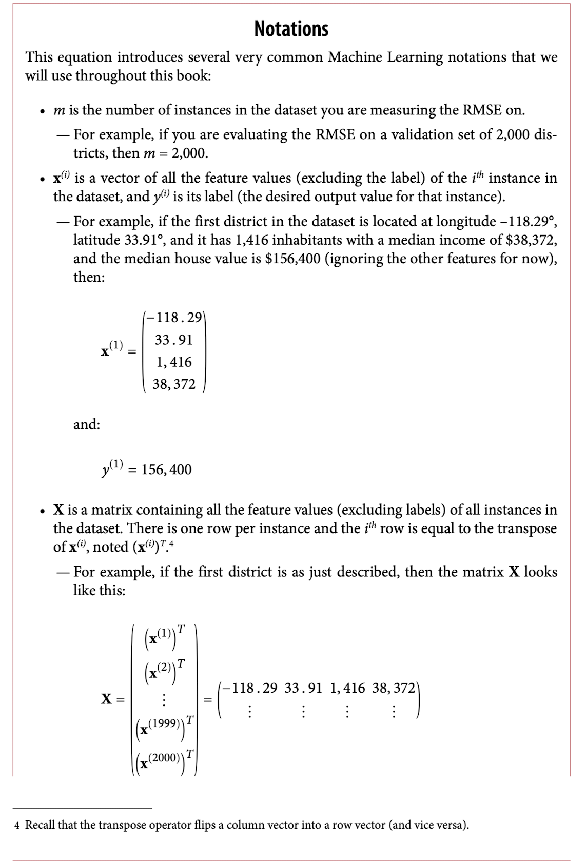
• Notations:

  • Lowercase italic font is used for scalar values, such as ( m ) or ( y^{(i)} ).
  • Lowercase bold font is used for vectors, such as ( \mathbf{x}^{(i)} ).
  • Uppercase bold font is used for matrices, such as ( \mathbf{X} ).

\

Pandas access type

Pandas offers various methods for accessing and manipulating data in a DataFrame. Here’s a comprehensive list of the primary ways to access and select data in pandas:

1. Accessing Columns:

• Single Column:

  df['column_name']   # Returns a Series
  df.column_name      # Dot notation (only for column names without spaces or special characters)

• Multiple Columns:

  df[['column1', 'column2']]  # Returns a DataFrame with the specified columns

2. Accessing Rows:

• Single Row by Index:

  df.iloc[0]    # Accesses the first row by integer index (returns a Series)
  df.loc[0]     # Accesses the row with index label 0 (if index is labeled numerically)

• Multiple Rows:

  df.iloc[0:3]     # Accesses the first three rows by integer index
  df.loc[0:2]      # Accesses rows with index labels 0, 1, and 2 (if index is labeled numerically)

• Access by Boolean Mask:

  df[df['column_name'] > value]  # Access rows based on a condition

3. Accessing Cells:

• Single Cell by Row and Column Name:

  df.at[row_label, 'column_name']    # Faster lookup for single values using labels

• Single Cell by Row and Column Index:

  df.iat[row_index, column_index]    # Faster lookup for single values using integer positions

4. Slicing DataFrames:

• Slicing Rows and Columns:

  df.iloc[0:3, 0:2]    # Accesses the first three rows and first two columns (by position)
  df.loc[0:2, ['column1', 'column2']]  # Accesses rows with labels 0, 1, 2 and specified columns (by label)

5. Accessing by Boolean Indexing:

• Boolean Conditions on DataFrames:

  df[df['column_name'] == 'some_value']      # Rows where 'column_name' equals 'some_value'
  df[(df['column1'] > 5) & (df['column2'] < 3)]  # Multiple conditions using & (AND) or | (OR)

6. Using .query() for SQL-like Access:

• Query with Column Names:

  df.query('column_name == value')  # SQL-like syntax for accessing rows

• Complex Queries:

  df.query('column1 > 5 & column2 < 3')  # Use logical operators within query

7. Accessing Using .loc and .iloc:

• .loc: Label-based access for rows and columns.

  df.loc[row_label, 'column_name']          # Single row and single column by label
  df.loc[row_label, ['col1', 'col2']]       # Single row and multiple columns by labels
  df.loc[[row_label1, row_label2], :]       # Multiple rows by labels and all columns

• .iloc: Integer position-based access for rows and columns.

  df.iloc[row_index, column_index]          # Single row and single column by integer index
  df.iloc[row_index, [col_idx1, col_idx2]]  # Single row and multiple columns by integer indices
  df.iloc[[row_idx1, row_idx2], :]          # Multiple rows by integer indices and all columns

8. Accessing Using .xs() for Cross-Sectional Access:

• Useful for selecting data from multi-indexed DataFrames.

  df.xs(key='index_name', level='index_level')  # Access a cross-section of a multi-index DataFrame

9. Accessing with .loc and .iloc Combined with .at and .iat:

• Access Single Value Using .at:

  df.at[row_label, 'column_name']    # Label-based access for a single value

• Access Single Value Using .iat:

  df.iat[row_index, column_index]    # Integer position-based access for a single value

10. Using .get() Method:

• Similar to dictionary-style access, useful when you want to provide a default value if the column doesn’t exist.

  df.get('column_name', default_value)  # Returns the column if exists, else returns the default_value

11. Using .filter() Method:

• Filter by Columns or Index:

  df.filter(items=['col1', 'col2'], axis=1)      # Filter specific columns
  df.filter(like='prefix', axis=1)               # Select columns with 'prefix'
  df.filter(regex='regex_pattern', axis=1)       # Select columns matching a regex pattern
  df.filter(like='substring', axis=0)            # Select rows with index containing 'substring'

12. Using .loc with Index Slices (slice()):

• Selecting Ranges of Rows:

  df.loc[slice(start_label, end_label), :]   # Select rows within the specified range of labels

13. Using .sample() to Access Random Rows or Columns:

• Select Random Rows or Columns:

  df.sample(n=5)           # Select 5 random rows
  df.sample(frac=0.1)      # Select 10% of the rows randomly
  df.sample(n=3, axis=1)   # Select 3 random columns

These are the main data access methods for pandas DataFrames. Depending on your use case, you can choose the method that fits best for selecting or manipulating your data.

value_counts() is a powerful pandas method that provides a quick and easy way to get the frequency counts of unique values in a Series or column of a DataFrame. Below, I’ll provide examples and other similar tactics for summarizing, analyzing, and manipulating categorical and numerical data in pandas.

Example tactics for Dataframe discovery

1. .value_counts() Usage

• Counting Unique Values in a Column:

  housing['ocean_proximity'].value_counts()

  This will display the frequency of each unique category in the ocean_proximity column.

• Example Output:

  NEAR BAY     3
  INLAND       2
  NEAR OCEAN   1
  Name: ocean_proximity, dtype: int64
  

• Sort and Normalize:

  housing['ocean_proximity'].value_counts(normalize=True)  # Show percentages instead of counts
  housing['ocean_proximity'].value_counts(sort=False)      # Prevent sorting of the values

2. .unique() and .nunique() for Unique Value Analysis

• Finding Unique Values:

  housing['ocean_proximity'].unique()  # Returns an array of unique values in the column

  • Output:

    array(['NEAR BAY', 'INLAND', 'NEAR OCEAN'], dtype=object)
    

• Counting Unique Values:

  housing['ocean_proximity'].nunique()  # Returns the number of unique values

  • Output:

    3
    

3. .count() for Counting Non-NA Values

• Count Non-NA/Null Values:

  housing['ocean_proximity'].count()  # Counts only non-null values in the column

• Count Non-NA/Null Values Across the DataFrame:

  housing.count()  # Counts non-null values for each column in the DataFrame

4. .describe() for Summary Statistics

• Generate Summary Statistics for Categorical and Numerical Columns:

  housing['ocean_proximity'].describe()  # Provides count, unique, top, and frequency for categorical columns
  housing.describe()                     # Summary statistics for numerical columns (mean, std, min, etc.)

5. .groupby() for Grouping and Aggregating Data

• Group and Count:

  housing.groupby('ocean_proximity').size()  # Similar to value_counts, but more flexible

• Group and Compute Other Statistics:

  housing.groupby('ocean_proximity')['median_house_value'].mean()  # Average house value by proximity
  housing.groupby('ocean_proximity').agg({'median_house_value': 'mean', 'population': 'sum'})  # Multiple aggregations

6. .crosstab() and .pivot_table() for Contingency Tables

• Cross Tabulation:

  pd.crosstab(housing['ocean_proximity'], housing['housing_median_age'])  # Frequency table of two variables

• Pivot Table:

  housing.pivot_table(values='median_house_value', index='ocean_proximity', columns='housing_median_age', aggfunc='mean')

7. .mode() for Finding the Most Frequent Values

• Get the Most Frequent Value in a Column:

  housing['ocean_proximity'].mode()  # Returns the mode (most common value)

8. .apply() for Applying Functions Across Columns or Rows

• Applying a Custom Function to a Column:

  housing['median_income_category'] = housing['median_income'].apply(lambda x: 'High' if x > 5 else 'Low')

  This creates a new column based on a condition applied to each value in the median_income column.

9. .map() and .replace() for Value Mapping

• Map Values Using a Dictionary:

  proximity_map = {'NEAR BAY': 'Close to Bay', 'INLAND': 'Inland Area', 'NEAR OCEAN': 'Close to Ocean'}
  housing['ocean_proximity'] = housing['ocean_proximity'].map(proximity_map)

• Replace Values Using .replace():

  housing['ocean_proximity'].replace({'Close to Bay': 'Bay Area'}, inplace=True)

10. .isin() for Filtering by Multiple Values

• Filter Rows Based on a List of Values:

  housing[housing['ocean_proximity'].isin(['NEAR BAY', 'INLAND'])]  # Rows where 'ocean_proximity' is 'NEAR BAY' or 'INLAND'

11. .cut() and .qcut() for Binning Continuous Data

• Binning Continuous Data into Categories:

  housing['income_bin'] = pd.cut(housing['median_income'], bins=[0, 2, 4, 6, 8], labels=['Low', 'Mid', 'High', 'Very High'])

• Quantile-based Binning:

  housing['income_quantile'] = pd.qcut(housing['median_income'], q=4)  # Divides data into 4 equal-sized bins

12. .rank() and .sort_values() for Ranking and Sorting

• Ranking Values:

  housing['income_rank'] = housing['median_income'].rank()

• Sorting by Column:

  housing.sort_values(by='median_house_value', ascending=False)  # Sort DataFrame by house value in descending order

13. .duplicated() and .drop_duplicates() for Managing Duplicates

• Identify Duplicates:

  housing.duplicated(subset='ocean_proximity')  # Returns a boolean Series indicating duplicates

• Remove Duplicates:

  housing.drop_duplicates(subset='ocean_proximity', inplace=True)  # Removes duplicate rows based on 'ocean_proximity'

14. .corr() for Correlation Analysis

• Correlation Between Numerical Columns:

  housing.corr()  # Returns correlation matrix for numerical columns

15. .plot() for Visualizing Value Counts

• Plot Value Counts:

  housing['ocean_proximity'].value_counts().plot(kind='bar')  # Visualize value counts as a bar plot

These methods and tactics provide a comprehensive approach to analyzing and manipulating data in pandas DataFrames, similar to how you would use .value_counts() to understand the distribution of categorical variables.

Data snooping bias

Data snooping bias (also known as data leakage or look-ahead bias) occurs when a machine learning model is inadvertently trained or evaluated using information that would not be available at prediction time, thereby leading to overly optimistic performance estimates. This typically happens when data that should be kept separate (such as training, validation, and test data) is somehow shared or influenced during the model development process.

Causes of Data Snooping Bias:

1. Using Test Data in Model Selection or Hyperparameter Tuning:

   • If the test data is used multiple times to select models or tune hyperparameters, the model’s performance will be biased because it has indirectly “seen” the test data during training.

2. Feature Engineering Using Future Information:

   • Creating features using information that would only be available in the future or that would be known after the event being predicted.

3. Leakage Through Data Preparation:

   • Sharing information between training and test sets during data preparation steps, such as normalizing or scaling based on the entire dataset instead of just the training set.

4. Unintentional Data Overlap:

   • Overlapping data in different subsets (e.g., using the same samples in training and test sets) or using variables that are directly correlated with the target variable in a way that would not be present during deployment.

Consequences of Data Snooping Bias:

• Overestimated Performance: The model’s performance on validation or test data may appear much better than it will be in real-world scenarios, leading to false confidence in the model.
• Poor Generalization: Since the model is essentially overfitting on the information it shouldn’t have access to, it will not generalize well to truly unseen data.

Example of Data Snooping Bias:

Suppose you are building a model to predict whether a stock’s price will rise or fall based on historical data. If you include information about whether the stock price rose or fell in the next month as part of your feature set, your model will achieve very high accuracy. However, this is a clear example of data snooping bias, as it uses future information that wouldn’t be available in a real-world setting.

How to Avoid Data Snooping Bias:

1. Separate Data Properly:

   • Maintain strict separation between training, validation, and test sets.
   • Never use the test set for model selection or hyperparameter tuning.

2. Avoid Using Future Information:

   • Do not include features in your model that would not be known at the time of prediction.

3. Create Training Pipelines:

   • Use separate pipelines for data preparation to avoid data leakage between training and testing phases (e.g., scaling based on training data only).

4. Cross-Validation:

   • Use cross-validation correctly to ensure that data leakage is minimized and that the model is evaluated fairly.

5. Be Cautious with Time Series Data:

   • When working with time series data, ensure that you don’t use future data points in training that wouldn’t be available at the prediction time.

In summary, data snooping bias occurs when the model is trained or validated using information that would not be available at prediction time, leading to misleading performance metrics. This bias must be carefully avoided to ensure that the model’s performance is reliable and realistic.

Explanation of StratifiedShuffleSplit

[StratifiedShuffleSplit] is a cross-validation strategy provided by sklearn that splits the data into training and testing sets while preserving the distribution of a specified class or feature variable. This technique is especially useful when dealing with imbalanced datasets, as it ensures that each subset (training and testing) maintains the same proportion of class labels as the original dataset.

Why Use StratifiedShuffleSplit?

• Maintains Class Distribution: Ensures that the train and test sets have the same proportion of classes as the original dataset. This is crucial when the target classes are imbalanced.
• Improved Model Evaluation: By preserving the class distribution, you can get a more reliable evaluation of your model’s performance.
• Prevents Bias in Small Datasets: Avoids the issue of certain classes being overrepresented or underrepresented in training or testing data.

Parameters of StratifiedShuffleSplit

• n_splits: Number of re-shuffling and splitting iterations (default is 10).
• test_size or train_size: Proportion or absolute number of test or train samples.
• random_state: Controls the shuffling for reproducibility.

Example: Using StratifiedShuffleSplit in Python

Below is an example of how to use StratifiedShuffleSplit with a dataset:

from sklearn.model_selection import StratifiedShuffleSplit
import pandas as pd
 
# Sample data
data = {
    'feature1': [10, 20, 30, 40, 50, 60, 70, 80, 90, 100],
    'feature2': [1, 2, 3, 4, 5, 6, 7, 8, 9, 10],
    'target': ['A', 'B', 'A', 'B', 'A', 'B', 'A', 'B', 'A', 'B']
}
 
# Create a DataFrame
df = pd.DataFrame(data)
 
# Define features and target
X = df[['feature1', 'feature2']]
y = df['target']
 
# Create a StratifiedShuffleSplit object
strat_split = StratifiedShuffleSplit(n_splits=1, test_size=0.2, random_state=42)
 
# Split the data into training and testing sets
for train_index, test_index in strat_split.split(X, y):
    X_train, X_test = X.iloc[train_index], X.iloc[test_index]
    y_train, y_test = y.iloc[train_index], y.iloc[test_index]
 
# Display the results
print("Train Set:")
print(X_train)
print(y_train)
print("\nTest Set:")
print(X_test)
print(y_test)

Output:

Train Set:
   feature1  feature2
5        60         6
2        30         3
4        50         5
3        40         4
8        90         9
9       100        10
0        10         1
1        20         2

5    B
2    A
4    A
3    B
8    A
9    B
0    A
1    B
Name: target, dtype: object

Test Set:
   feature1  feature2
7        80         8
6        70         7

7    B
6    A
Name: target, dtype: object

Explanation:

• In this example, the original dataset contains equal proportions of classes A and B.
• StratifiedShuffleSplit is applied with a single split (n_splits=1) and a test_size of 20% (test_size=0.2).
• After splitting, both the training and test sets maintain the same proportion of class labels A and B.

Additional Parameters and Methods:

• split(X, y): Splits X (features) and y (target labels) into training and testing indices while maintaining the class distribution.
• n_splits: Number of re-shuffling and splitting iterations (default is 10).
• random_state: Controls the randomness of the split for reproducibility.
• test_size: The proportion of the dataset to include in the test split.

When to Use StratifiedShuffleSplit

• Imbalanced Datasets: When the target variable has an uneven distribution of classes.
• Classification Tasks: Especially useful for classification problems where preserving class distribution is crucial.
• Small Datasets: Helps prevent bias and maintains a balanced representation of classes in training and testing sets.

Summary

StratifiedShuffleSplit is a powerful tool to ensure that your training and testing sets maintain the same distribution of classes as the original dataset, making it an ideal choice for classification problems with imbalanced classes.

Standard Correlation Coefficient (Pearson’s r)

The standard correlation coefficient, also known as Pearson’s correlation coefficient or Pearson’s r, measures the linear relationship between two continuous variables. It indicates the strength and direction of the relationship, ranging from -1 to +1.

Formula

The formula for Pearson’s r is:

$$r=\frac{{\sum }_{i=1}^n(x_i-\bar{x})(y_i-\bar{y})}{\sqrt{{\sum }_{i=1}^n(x_i-\bar{x}{)}^2}\cdot \sqrt{{\sum }_{i=1}^n(y_i-\bar{y}{)}^2}}$$

Where:

• \ ( x_i ) and ( y_i ) are the individual sample points of variables ( x ) and ( y ).
• \ ( \bar{x} ) and ( \bar{y} ) are the mean values of variables ( x ) and ( y ).
• \ ( n ) is the number of sample points.

Interpretation

• Range: The correlation coefficient ( r ) ranges from -1 to +1:

  • ( r = 1 ): Perfect positive linear correlation (as one variable increases, the other increases proportionally).
  • ( r = -1 ): Perfect negative linear correlation (as one variable increases, the other decreases proportionally).
  • ( r = 0 ): No linear correlation (the variables do not have any linear relationship).

• Positive Correlation: If ( r ) is positive, it indicates that as one variable increases, the other tends to increase.

• Negative Correlation: If ( r ) is negative, it indicates that as one variable increases, the other tends to decrease.

• Magnitude of Correlation:

  • The closer ( r ) is to +1 or -1, the stronger the linear relationship between the variables.
  • The closer ( r ) is to 0, the weaker the linear relationship.

Assumptions of Pearson’s Correlation

1. Linearity: Assumes a linear relationship between the variables.
2. Continuous Data: Both variables should be continuous.
3. Normality: The variables should be approximately normally distributed.
4. No Outliers: Pearson’s r is sensitive to outliers, which can skew the results.

Example in Python

You can use pandas or scipy to calculate Pearson’s correlation coefficient in Python. Here’s an example using pandas:

import pandas as pd
 
# Sample data
data = {
    'height': [150, 160, 170, 180, 190],
    'weight': [50, 55, 60, 70, 80]
}
 
# Create a DataFrame
df = pd.DataFrame(data)
 
# Calculate Pearson's correlation coefficient
correlation_matrix = df.corr(method='pearson')
print("Pearson's r correlation matrix:\n", correlation_matrix)
 
 

OUTPUT:

Pearson’s r correlation matrix: height weight height 1.000000 0.981981 weight 0.981981 1.000000