Generative Modeling
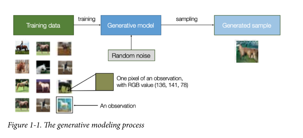
A generative model describes how a dataset is generated, in terms of a probabilistic model. By sampling from this model, we are able to generate new data.
First, we require a dataset consisting of many examples of the entity we are trying to generate. This is known as the training data, and one such data point is called an observation.
generative model must also be probabilistic rather than deterministic. If our model is merely a fixed calculation, such as taking the average value of each pixel in the dataset, it is not generative because the model produces the same output every time. The model must include a stochastic (random) element that influences the individual samples generated by the model.
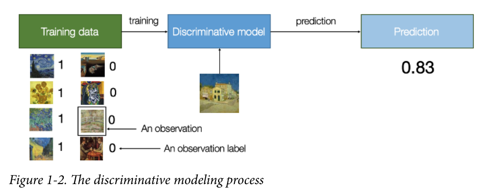
One key difference is that when performing discriminative modeling, each observa‐ tion in the training data has a label.
Discriminative modeling estimates p( y | x) —the probability of a label y given observa‐ tion x.
Generative modeling estimates p(x) —the probability of observing observation x. If the dataset is labeled, we can also build a generative model that estimates the distri‐ bution p(x | y) .
In other words, discriminative modeling attempts to estimate the probability that an observation x belongs to category y. Generative modeling doesn’t care about labeling observations. Instead, it attempts to estimate the probability of seeing the observation at all.
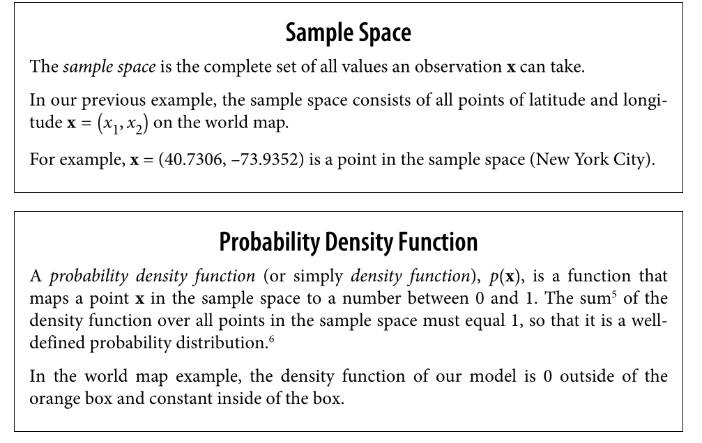
sample space, density function, parametric modeling, maximum likelihood estimation
Generative Modeling Challenges • How does the model cope with the high degree of conditional dependence between features? • How does the model find one of the tiny proportion of satisfying possible gener‐ ated observations among a high-dimensional sample space?
The fact that deep learning can form its own features in a lower-dimensional space means that it is a form of representation learning. It is important to understand the key concepts of representation learning before we tackle deep learning in the next chapter.
Representation Learning
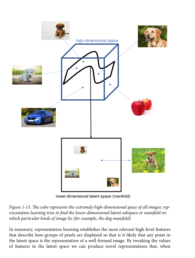
The core idea behind representation learning is that instead of trying to model the high-dimensional sample space directly, we should instead describe each observation in the training set using some low-dimensional latent space and then learn a mapping function that can take a point in the latent space and map it to a point in the original domain. In other words, each point in the latent space is the representation of some high-dimensional image.
Variational Autoencoder VAE
• An encoder network that compresses high-dimensional input data into a lower- dimensional representation vector • A decoder network that decompresses a given representation vector back to the original domain
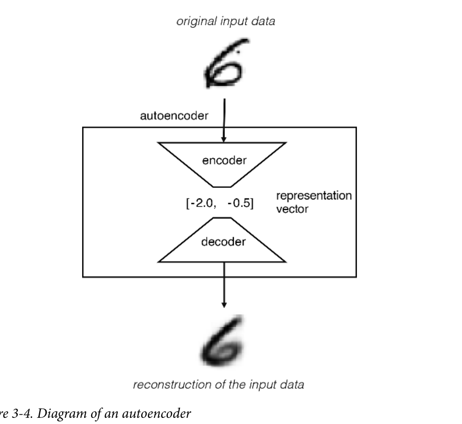
The network is trained to find weights for the encoder and decoder that minimize the loss between the original input and the reconstruction of the input after it has passed through the encoder and decoder.
Autoencoders can be used to generate new data through a process called “autoencoder decoding” or “autoencoder sampling.” Autoencoders are neural network models that learn to encode input data into a lower-dimensional representation (latent space) and then decode it back to reconstruct the original input. This reconstruction process can also be used to generate new data that resembles the patterns learned during training.
Here’s a general approach to using an autoencoder for data generation:
-
Train an Autoencoder: Start by training an autoencoder on a dataset of your choice. The autoencoder consists of an encoder network that maps the input data to a lower-dimensional latent space and a decoder network that reconstructs the original input from the latent space representation.
-
Latent Space Exploration: After training, you can explore the learned latent space by sampling points from it. Randomly generate vectors or sample from a probability distribution to create latent space representations.
-
Decoding: Pass the sampled latent space representations through the decoder network to generate new data. The decoder will transform the latent space representations back into the original data space, generating synthetic data that resembles the patterns learned during training.
-
Control Generation: By manipulating the values of the latent space representations, you can control the characteristics of the generated data. For example, you can interpolate between two latent space points to create a smooth transition between two data samples or explore specific directions in the latent space to generate variations of a particular feature.
It’s important to note that the quality of the generated data heavily depends on the quality of the trained autoencoder and the complexity of the dataset. Autoencoders are most effective when trained on datasets with clear patterns and structure.
There are variations of autoencoders, such as variational autoencoders (VAEs), that introduce probabilistic components and offer more control over the generation process. VAEs can generate data that follows a specific distribution by sampling latent variables from the learned distributions.
Remember that the generated data is synthetic and may not perfectly match the real data distribution. It’s crucial to evaluate the generated samples and assess their usefulness for your specific application.
Variational autoencoders solve these problems, by introducing randomness into the model and constraining how points in the latent space are distributed. We saw that with a few minor adjustments, we can transform our autoencoder into a variational autoencoder, thus giving it the power to be a generative model.
Finally, we applied our new technique to the problem of face generation and saw how we can simply choose points from a standard normal distribution to generate new faces. Moreover, by performing vector arithmetic within the latent space, we can ach‐ ieve some amazing effects, such as face morphing and feature manipulation. With these features, it is easy to see why VAEs have become a prominent technique for gen‐ erative modeling in recent years.