statistics #numpy #pandas

What is statistics?

The field of statistics - the practice and study of collecting and analyzing data A summary statistic - a fact about or summary of some data

See PDF 1 link See PDF 2 link See PDF 3 link See PDF 4 link

Types of statistics

Descriptive statistics Describe and summarize data 50% of friends drive to work
Inferential statistics Use a sample of data to make inferences about a larger population What percent of people drive to work?

Types of data

Types of Data	Nature	Examples
Numeric (Quantitative)	Continuous (Measured)	Airplane speed (e.g., 600 mph)
		Time spent waiting in line (e.g., 20 minutes)
--------------------------	-------------------	-------------------------------------------
	Discrete (Counted)	Number of pets (e.g., 2 dogs)
		Number of packages shipped (e.g., 10 packages)
--------------------------	-------------------	-------------------------------------------
Categorical (Qualitative)	Nominal (Unordered)	Marital status (e.g., Married/Unmarried)
		Country of residence (e.g., USA, Canada)
--------------------------	-------------------	-------------------------------------------
	Ordinal (Ordered)	Educational level (e.g., Bachelor’s Degree)
		Socioeconomic status (e.g., Middle Class)
		Customer satisfaction rating (e.g., 4 out of 5)
		Likert Scale (e.g., Agree)

Categorical data can be represented as numbers

Nominal (Unordered) Married/unmarried ( 1 / 0 ) Ordinal (Ordered) Strongly disagree ( 1 ) Somewhat disagree ( 2 ) Neither agree nor disagree ( 3 ) Somewhat agree ( 4 ) Strongly agree ( 5 )

Why data type matter ?

Data type matters in various aspects of data analysis and decision-making for several reasons:

Data Representation: Different data types require different methods of representation. Understanding the data type helps in choosing the appropriate data structures for storage and analysis. For example, numeric data may be stored as floating-point numbers, while categorical data may be stored as strings or integers.
Data Analysis Techniques: The type of data determines which statistical or analytical techniques are suitable for analysis. For instance, you would use different methods to analyze numeric data compared to categorical data. Using the wrong analysis method can lead to incorrect results and conclusions.
Data Visualization: Data type influences how data is visualized. Scatter plots and histograms are useful for numeric data, while bar charts and pie charts are often used for categorical data. Understanding the data type helps in creating effective data visualizations.
Data Preprocessing: Data type affects data preprocessing steps. For example, missing values may need to be handled differently for numeric and categorical data. Data transformation techniques, such as one-hot encoding for categorical data, are specific to data types.
Modeling and Machine Learning: In machine learning, the data type of features and the target variable is crucial. Algorithms have specific requirements and assumptions about data types. For example, linear regression typically works with numeric data, while decision trees can handle both numeric and categorical data.
Interpretation: The interpretation of results depends on data type. For example, when interpreting correlation coefficients between two numeric variables, you can make statements about the strength and direction of the relationship. Interpreting results from logistic regression for categorical data involves odds ratios and probabilities.
Data Quality and Validation: Understanding data type is essential for data validation and data quality checks. It helps in identifying inconsistencies or errors in the data. For instance, if a numeric field contains non-numeric values, it could be a data quality issue.
Data Integration: When combining data from multiple sources, understanding data types helps in data integration. Mismatched data types can lead to integration challenges and data transformation requirements.
Decision-Making: Ultimately, the correct interpretation of data and informed decision-making rely on understanding data types. Making decisions based on misinterpreted or mishandled data can have significant consequences.

In summary, data type matters because it affects how data is treated, analyzed, and interpreted. A clear understanding of data types is fundamental for effective data analysis and informed decision-making in various domains, including business, science, and technology.

import pandas as pd
import numpy as np
data = {
    "Species": [
        "African Elephant", "Giraffe", "Lion", "Hippopotamus", "Gorilla",
        "Cheetah", "Kangaroo", "Koala", "Brown Bat", "Dolphin",
        "Human", "Hedgehog", "Sloth", "Raccoon", "Dog", "Cat", "Mouse"
    ],
    "Class": ["Mammal"] * 17,
    "Hours of Sleep per Day": [
        3.5, 4.6, 13.5, 4.5, 9.9,
        12.1, 4.8, 18.0, 19.9, 4.0,
        7.0, 10.0, 14.4, 12.5, 12.0, 12.0, 12.5
    ]
}
 
# Create a pandas DataFrame from the dictionary
mammal_sleep_df = pd.DataFrame(data)
 
# Print the DataFrame
print(mammal_sleep_df)
 
# print mean of data
print(np.mean(mammal_sleep_df['Hours of Sleep per Day']))

histogram

The histogram is a popular graphing tool. It is used to summarize discrete or continuous data that are measured on an interval scale. It is often used to illustrate the major features of the distribution of the data in a convenient form. It is also useful when dealing with large data sets (greater than 100 observations). It can help detect any unusual observations (outliers) or any gaps in the data.

See also Canadian statistics website link

mod #median #mean

You would use measures of central tendency (mean, median, and mode) in various situations in data analysis and statistics to summarize and understand the characteristics of a dataset. Here are some common scenarios when each measure is useful:

Mean:
- Use the mean when you want to find the average value of a dataset.
- It’s appropriate for data that is approximately normally distributed or symmetric, where the values are relatively evenly distributed around a central value.
- Be cautious when using the mean with data that has outliers, as outliers can significantly affect the mean.
Example: Calculating the average test score in a class.
Median:
- Use the median when you want to find the middle value of a dataset.
- It’s robust to outliers and resistant to extreme values, making it suitable for data with outliers or skewed distributions.
- Useful when you want to understand the central value that divides the data into equal halves.
Example: Determining the median income in a population.
Mode:
- Use the mode when you want to find the most frequently occurring value(s) in a dataset.
- It’s suitable for categorical data or discrete data with distinct categories.
- Can help identify the most common categories or values in a dataset.
Example: Identifying the most popular flavor of ice cream in a survey.

In practice, the choice of which measure to use depends on the nature of your data and the specific questions you want to answer:

If your data is roughly symmetric and free from outliers, the mean is often a good choice.
If your data is skewed or contains outliers, the median may provide a more representative central value.
For categorical or discrete data, the mode helps identify the most frequent category or value.

It’s also common to use a combination of these measures to gain a more comprehensive understanding of your data. Additionally, visualizations such as histograms, box plots, and scatter plots can provide valuable insights into the distribution and central tendency of your data.

import numpy as np
data = [10, 15, 20, 25, 30]
mean_value = np.mean(data)
print("Mean:", mean_value)
 
 
# FOR MEDIAN YOU NEED TO SORTED DATA
median_value = np.median(data)
sorted_data = sorted(data)
print("Median:", sorted_data)
 
from statistics import mode
 
data = [10, 15, 20, 25, 20, 30]
mode_value = mode(data)
print("Mode:", mode_value)
# when you using in dataframe
#msleep['vore'].value_counts()
# statistics.mode(msleep['vore'])

skew #leftskewed #rightskewed

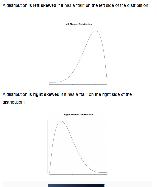
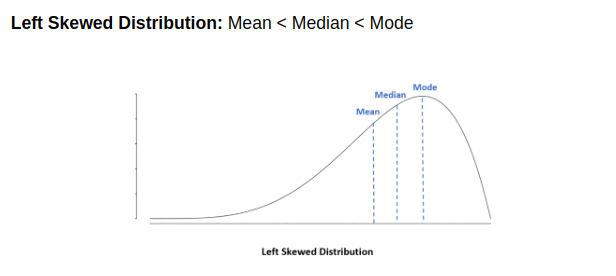
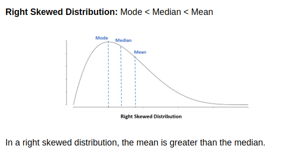
When dealing with skewed data, whether positively skewed (right-skewed) or negatively skewed (left-skewed), the choice between using the mean or the median as a measure of central tendency depends on the specific characteristics of the data and the goals of your analysis. Here are some guidelines:

Positively Skewed Data (Right-Skewed):
- In a positively skewed distribution, the tail of the data points extends to the right, meaning that there are relatively few extremely high values pulling the mean to the right.
- Use the median when you want a measure of central tendency that is less affected by extreme outliers or when you want to describe the typical value for the majority of the data.
- The mean can be significantly higher than the median in positively skewed data because it is influenced by the long tail of high values. If you use the mean, be aware that it may not accurately represent the central tendency for the majority of the data.
Negatively Skewed Data (Left-Skewed):
- In a negatively skewed distribution, the tail of the data points extends to the left, meaning that there are relatively few extremely low values pulling the mean to the left.
- Use the median when you want a measure of central tendency that is less affected by extreme outliers or when you want to describe the typical value for the majority of the data.
- Similar to positively skewed data, the mean can be significantly lower than the median in negatively skewed data because it is influenced by the long tail of low values. If you use the mean, it may not accurately represent the central tendency for the majority of the data.

In summary, for skewed data, it’s often a good practice to report both the mean and the median, along with other summary statistics, to provide a more complete picture of the data’s distribution. Additionally, visualizations like histograms or box plots can help you assess the skewness and understand the shape of the distribution, aiding in the choice of the appropriate measure of central tendency.

variance

Variance

Average distance from each data point to the data’s mean

import pandas as pd
 
# Sample DataFrame
data = {
    'A': [10, 15, 12, 8, 14],
    'B': [25, 30, 22, 18, 27],
    'C': [7, 11, 9, 5, 10]
}
 
df = pd.DataFrame(data)
 
# Calculate the variance using .var() method
variance_df = df['C'].var()
 
# Calculate the mean of column 'C'
mean_c = df['C'].mean()
 
# Calculate the squared differences from the mean
squared_diff = (df['C'] - mean_c) ** 2
 
# Calculate the variance manually
variance_manual = squared_diff.mean()
 
print("Variance for column 'C' using .var() method:", variance_df)
print("Variance for column 'C' (calculated manually):", variance_manual)
 
# Compare the results
if variance_df == variance_manual:
    print("The results match.")
else:
    print("The results do not match.")

What is ddof ?

In the expression np.var(msleep['sleep_total'], ddof=1), ddof stands for “Delta Degrees of Freedom.” It is a parameter used to specify the degrees of freedom correction when calculating the variance.

Degrees of freedom (DF) represent the number of values in the final calculation of a statistic that are free to vary. In the context of calculating the variance, degrees of freedom refer to the number of independent pieces of information used in the calculation. The concept is relevant when you are calculating sample variance, as opposed to population variance.

Here’s how ddof works in the context of variance calculation:

Population Variance (ddof=0): When you want to calculate the variance of an entire population (all available data points), you set ddof to 0. This is because you are using all the data points, and there are no degrees of freedom being “lost” due to estimation.

Example:
```
population_var = np.var(data, ddof=0)  # Calculate population variance
```
Sample Variance (ddof=1): When you are dealing with a sample (a subset of the population) and you want to estimate the variance of the entire population based on that sample, you set ddof to 1. This correction accounts for the loss of one degree of freedom when estimating the population variance from a sample.

Example:
```
sample_var = np.var(sample_data, ddof=1)  # Calculate sample variance
```

In most cases, when working with sample data, you’ll want to use ddof=1 to calculate the sample variance because it provides an unbiased estimate of the population variance. It accounts for the fact that you are estimating the population variance based on a sample and adjusts the calculation accordingly. However, if you’re working with a full population dataset, you can use ddof=0 to calculate the population variance directly.

Standard-deviation

Standard deviation

Formula

$\sigma={\sqrt {\frac {\sum(x_{i}-{\mu})^{2}}{N}}}$


$\sigma$	=	population standard deviation
	=	the size of the population
	=	each value from the population
$\mu$	=	the population mean

quantiles

Quantiles are values that divide a dataset into equal-sized subsets or intervals. They help us understand the distribution of data and identify specific data points that represent certain percentiles or proportions of the data.

Here are some common quantiles:

Quartiles divide the data into four equal parts, with three quartile values: Q1 (25th percentile), Q2 (50th percentile, or median), and Q3 (75th percentile).
Percentiles divide the data into 100 equal parts. The median is the 50th percentile (P50), and other percentiles like the 25th percentile (P25) and 75th percentile (P75) are commonly used.
Deciles divide the data into 10 equal parts, with values like the 10th decile (D10), 20th decile (D20), and so on.
Quintiles divide the data into 5 equal parts, with values like the 20th quintile (Q20), 40th quintile (Q40), and so on.

To calculate quantiles in Python, you can use libraries like NumPy or pandas. Here’s an example using NumPy:

import numpy as np
 
# Sample dataset
data = [12, 15, 18, 22, 25, 30, 32, 35, 40, 45, 50]
 
# Calculate quartiles (Q1, Q2, Q3)
q1 = np.percentile(data, 25)
q2 = np.percentile(data, 50)
q3 = np.percentile(data, 75)
 
print("Q1 (25th percentile):", q1)
print("Q2 (50th percentile, median):", q2)
print("Q3 (75th percentile):", q3)
 
# Calculate other percentiles (e.g., 10th and 90th percentiles)
p10 = np.percentile(data, 10)
p90 = np.percentile(data, 90)
 
print("P10 (10th percentile):", p10)
print("P90 (90th percentile):", p90)

In this code:

We have a sample dataset data containing 11 values.
We use np.percentile() from NumPy to calculate various quantiles and percentiles of the data. You specify the desired percentile as the second argument to the function.
We calculate quartiles (Q1, Q2, Q3) and percentiles (P10 and P90) in this example. You can adjust the percentiles according to your needs.

Running this code will display the calculated quantiles and percentiles for the given dataset. Quantiles are valuable for summarizing and understanding the distribution of data, especially in statistics and data analysis.

outliners

Outliers Outlier: data point that is substantially different from the others How do we know what a substantial difference is? A data point is an outlier if: data < Q1 − 1.5 × IQR or data > Q3 + 1.5 × IQR

In statistics, outliers are data points that are significantly different from the majority of the data in a dataset. They can be unusually high or low values compared to the rest of the data and can potentially skew statistical analyses or model results if not properly identified and handled.

One common method for identifying outliers is using the Interquartile Range (IQR) method, which you mentioned. The IQR is a measure of the spread or variability of the middle 50% of the data. Here’s how it works:

Calculate the IQR:
- Calculate the first quartile (Q1) and the third quartile (Q3) of the dataset.
- The IQR is defined as: [ IQR = Q3 - Q1 ]
Identify Outliers:
- Any data point that falls below [ Q1 - 1.5 \times IQR ] or above [ Q3 + 1.5 \times IQR ] is considered an outlier.

In other words, data points are considered outliers if they are more than 1.5 times the IQR away from either the lower quartile (Q1) or the upper quartile (Q3).

Here’s some Python code to identify outliers using the IQR method:

import numpy as np
 
# Sample dataset (replace with your own data)
data = [12, 15, 18, 22, 25, 30, 32, 35, 40, 45, 200]
 
# Calculate quartiles (Q1 and Q3)
q1 = np.percentile(data, 25)
q3 = np.percentile(data, 75)
 
# Calculate IQR
iqr = q3 - q1
 
# Define lower and upper bounds for identifying outliers
lower_bound = q1 - 1.5 * iqr
upper_bound = q3 + 1.5 * iqr
 
# Identify outliers
outliers = [x for x in data if x < lower_bound or x > upper_bound]
 
print("Outliers:", outliers)

In this code:

We calculate the first quartile (Q1) and third quartile (Q3) using np.percentile().
We calculate the IQR as the difference between Q3 and Q1.
We define the lower and upper bounds for identifying outliers as per the IQR method.
We identify outliers by iterating through the data and checking if each data point falls outside the defined bounds.

Running this code will identify and print the outliers in the given dataset. Outliers are important to be aware of because they can have a significant impact on statistical analyses and may require special treatment in data analysis and modeling processes.

pandas dataframe
In [1]:

food_consumption.head()  

Out[1]:

Unnamed: 0 country food_category consumption co2_emission 0 1 Argentina pork 10.51 37.20 1 2 Argentina poultry 38.66 41.53 2 3 Argentina beef 55.48 1712.00 3 4 Argentina lamb_goat 1.56 54.63 4 5 Argentina fish 4.36 6.96

# Calculate the quartiles of co2_emission
 
print(np.quantile(food_consumption['co2_emission'], [0, 0.25, 0.5, 0.75, 1]))

uniformcdf

The uniform.cdf() function is typically associated with a probability distribution called the uniform distribution. In probability theory and statistics, the uniform distribution is a continuous probability distribution that describes a random variable with equal probability of taking any value within a specified range. The uniform.cdf() function is used to calculate the cumulative distribution function (CDF) of a uniform distribution.

Here’s an explanation of the terms and concepts involved:

Uniform Distribution: In a uniform distribution, all values within a given range have the same probability of occurring. The probability density function (PDF) of the uniform distribution is flat within the specified range and zero outside that range.
Cumulative Distribution Function (CDF): The CDF of a random variable is a function that gives the probability that the random variable takes on a value less than or equal to a specified value. In the case of the uniform distribution, the CDF represents the cumulative probability that a random variable falls within a certain interval.

The uniform.cdf(x, loc, scale) function takes three parameters:

x: The value at which you want to calculate the CDF.
loc: The lower bound of the uniform distribution (the minimum possible value). Default is 0.
scale: The range of the uniform distribution (the difference between the upper bound and lower bound). Default is 1.

The uniform.cdf(x, loc, scale) function returns the cumulative probability that a random variable following a uniform distribution is less than or equal to x.

Here’s an example in Python using the SciPy library:

from scipy.stats import uniform
 
# Define parameters of the uniform distribution
lower_bound = 0
upper_bound = 10
scale = upper_bound - lower_bound
 
# Calculate the CDF at x = 5
x = 5
cdf_value = uniform.cdf(x, loc=lower_bound, scale=scale)
 
print(f"CDF at x = {x}: {cdf_value:.4f}")

In this example, we define a uniform distribution with a lower bound of 0 and an upper bound of 10 (resulting in a range of 10 - 0 = 10). We then calculate the CDF at x = 5, which gives us the cumulative probability that a random variable following this uniform distribution is less than or equal to 5. The result will be printed to the console.

#uniform.rvs()

Here’s a more specific explanation:

uniform.rvs() Function: This function is part of the SciPy library and is used to generate random variates (samples) from a uniform distribution.
Uniform Distribution: A uniform distribution is a probability distribution where all values within a specified interval have equal probability. In other words, if you were to plot the probability density function (PDF) of a uniform distribution, it would look like a flat line within the specified interval, indicating that all values in that interval are equally likely to occur.
Random Variates: “Random variates” are simply random values or samples drawn from a probability distribution. When you use uniform.rvs(), you are generating random values that follow the pattern of a uniform distribution.
Uniformity: The term “uniform” in this context emphasizes that the distribution of random values is even or consistent across the specified interval, with no particular values being favored over others.

Here’s an example using uniform.rvs() to generate random variates from a uniform distribution:

from scipy.stats import uniform
 
# Define the parameters of the uniform distribution
lower_bound = 0  # Lower bound of the interval
upper_bound = 10  # Upper bound of the interval
 
# Generate a random sample of size 5 from the uniform distribution
random_sample = uniform.rvs(loc=lower_bound, scale=upper_bound - lower_bound, size=5)
 
# Print the generated random sample
print(random_sample)

In this example, uniform.rvs() is used to generate random variates within the interval [0, 10] (inclusive of 0 and 10), and each value within that interval has an equal chance of being selected, reflecting the uniform distribution.

binomial distribution

The normal distribution

normcdf

The norm.cdf() function is part of the SciPy library and is used to calculate the cumulative distribution function (CDF) of a normal (Gaussian) distribution. The normal distribution is a continuous probability distribution that is often used in statistics due to its prevalence in various natural phenomena. The CDF of a normal distribution gives the probability that a random variable following that distribution is less than or equal to a specified value.

Here’s an explanation of the terms and concepts involved:

Normal Distribution (Gaussian Distribution):
- The normal distribution is a symmetric, bell-shaped probability distribution characterized by two parameters: mean (μ) and standard deviation (σ).
- The probability density function (PDF) of the normal distribution is given by the famous bell curve formula.
Cumulative Distribution Function (CDF):
- The CDF of a probability distribution is a function that gives the cumulative probability of a random variable being less than or equal to a specified value.
- For the normal distribution, the CDF is calculated by integrating the PDF from negative infinity to the specified value.
norm.cdf(x, loc, scale):
- The norm.cdf() function takes three parameters:
  - x: The value at which you want to calculate the CDF.
  - loc (optional): The mean (μ) of the normal distribution. Default is 0.
  - scale (optional): The standard deviation (σ) of the normal distribution. Default is 1.
- It returns the cumulative probability that a random variable following a normal distribution with the specified mean and standard deviation is less than or equal to x.

Here’s an example of how to use norm.cdf() in Python:

from scipy.stats import norm
 
# Define parameters of the normal distribution
mean = 0  # Mean (μ)
std_dev = 1  # Standard deviation (σ)
 
# Calculate the CDF at x = 1
x = 1
cdf_value = norm.cdf(x, loc=mean, scale=std_dev)
 
print(f"CDF at x = {x}: {cdf_value:.4f}")

In this example:

We import the norm module from the SciPy library.
We define the parameters of the normal distribution, including the mean (loc) and standard deviation (scale).
We use norm.cdf() to calculate the cumulative probability that a random variable from this normal distribution is less than or equal to x = 1.

The result represents the probability that a random variable from the specified normal distribution is less than or equal to 1.

Erdem's Second Brain

Explorer

Intro Statistics in Python